
 |
| Input Settings |
After selecting the two variables of interest, the user selects a radio button for the curve bounding method, “range limited” (user defined geometry range), or “constant margin of safety”.
Range Controlled:
After selecting this method, the user inputs a X range and Y range into the variable boxes, see Input Settings figure above. The X and Y range are mapped linearly with respect to each other. LugCalc™ will generate the margin of safety solution for all points in the defined range. The line point density field defines how many points in the range will be solved for. This solution is relatively fast because LugCalc™ is only repeating the margin of safety calculation for as many times as you specify in the line point density field. This tool is beneficial to the user who is trying to understand how the margin of safety changes with geometry modification. This tool is also valuable for MRB engineers trying to understand what happens with a lug margin of safety as the lug bore is reworked in repair.
 |
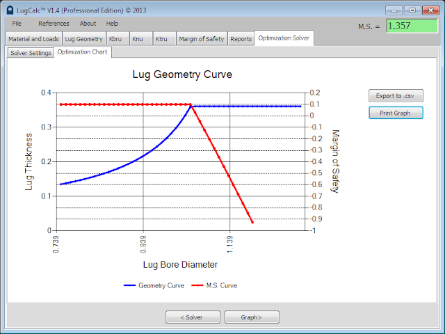
| Range Limited Solution Graph |
In the above example graph, it can be seen that the lug geometry range gives a positive value for M.S. up to a lug bore diameter of ~0.913 and lug thickness of ~0.1. Also the non-linear behavior of margin of safety is noticeable in the slight upward bend of the margin of safety line (red).
Constant Margin of Safety:
After selecting this method, the user inputs a number range for the X range variable previously selected. The start (min) X value is commonly the initial value in geometry tab for the X variable. Next, a start value is given for the Y value to initiate the solve. This value is typically the nominal value for Y used in the geometry tab. Finally, the user inputs a margin of safety value they want to hold constant.
 |
| Constant Margin of Safety Input |
The line point density value functions exactly as it does for range controlled solve except increasing this value can significantly increase the solve time. LugCalc™ uses a search algorithm to minimize the variables for X and Y to a constant margin of safety. The search algorithm has to be implemented for as many times as the line point density value is set. It is sometimes advisable to increase the line point density if the predefined range has a inflection point where it becomes impossible to hold the margin of safety constant for the defined X range. The progress bar at the bottom of the window will give you an idea of how long the solution will take.
 |
| Constant Margin of Safety Graph |
In the above graph, the margin of safety was held constant at 0.1. The X axis variable defines the range of solutions and the Y axis variable is minimized. The Y axis variable is always the minimized variable, therefore, adjust the Y axis variable as needed depending on the solution required.
The constant margin of safety solver is a powerful tool for optimizing lug size to static strength requirements. It helps the user understand exactly what margin the lug can hold constant or exactly where the lug will drop below a zero margin of safety.
In the following example, it can be seen that the solver holds the margin of safety constant up to a certain bore diameter (~1.0), at this point the solver holds the minimized variable (lug thickness) constant as the lug bore is increased over the defined range because it is no longer possible to maintain the goal margin.
 |
| Solver Inflection Example |
Either solve method can be used to generate optimized lug geometry or rework curves for lug joints. The method used depends on the goal of the design.
From the chart tab, the user can print the result or export the data to a .csv file for incorporation into a report or repair manual.